|
|
#19. The MagnetopauseThe magnetic boundary between the Earth's field and the solar wind, named the magnetopause, has a bullet-shaped front, gradually changing into a cylinder. Its cross-section is approximately circular.
|
|
|
|
| The tight bond between particles and field lines can sometimes be broken, e.g. when the particles undergo collisions or when the plasma flows through a "neutral point" where the field's intensity drops to zero. On a plot of magnetic field lines, such points stand out as the ones where field lines appear to intersect each other. Intersecting field lines seem to make no sense: how can the magnetic field point in two directions at once? If our plots nevertheless show such points, the intensity of the magnetic force at them must be zero, so that the direction of that force is irrelevant.
|
|
For example, one gets such points when one plots the field line configuration inside a magnetopause which perfectly confines all of the Earth's field lines (drawing above). There will be two such points, known as the cusps of the magnetosphere, and they mark the separation between lines going sunward and those going tailward. When spacecraft were actually sent to the cusp region--the European HEOS 1 and HEOS 2 (1968, 1972) and the University of Iowa's "Hawkeye" (1974)--they seemed to observe a disordered magnetic field, weak but not zero. The absence of a strong field to hold off the solar wind means that these are "weak spots" on the magnetopause, and solar wind plasma penetrates there to fill two funnel-shaped regions. Some of the plasma particles travel all the way to the top of the atmosphere, where their collisions produce a red auroral glow.
The Open Magnetosphere |
| A feature of simple neutral points is that the magnetic fields flanking them have opposite directions (drawing). Field lines just inside the "nose" of the magnetopause point northward. On the other hand, at times when the IMF has a southward slant, as its field lines become draped against the nose (drawing) they have a generally southward orientation.
|
|
The northward flowing group would migrate to line "3" in the drawing, an "open magnetic field line" linking Earth to interplanetary space. A short time later the field line linking those particles will occupy position "4", then "5". Dungey proposed that the process was reversed at some distant neutral point (or neutral line) "6" in the far tail, as illustrated here by a figure adapted from his original article. There the interplanetary line halves were reunited and flowed away, and the ends connected to Earth were also joined up again. Since the nose of the magnetosphere (on the average) maintains its position and is not "worn away" by the reconnection process, the magnetic field lines swept into the tail, and the plasma particles strung along them, must somehow flow back towards Earth, inside the magnetosphere. This (according to Dungey) explained the large-scale sunward flow of the tail, deduced from auroral motions and flows in the polar ionsphere, on field lines which extended into the tail. Dungey's process of "magnetic reconnection" is expected to increase the flow of energy from the solar wind to the magnetosphere, by establishing a direct field-line link between the two. It does, however, require a southward slant of interplanetary magnetic field lines, a condition which only exists about half the time. In 1966, soon after regular observations of the IMF began, a student of Dungey, Don Fairfield, did in fact note a strong correlation between such southward slants and the storminess of the magnetic field ("magnetic activity"). Nowadays "southward IMF" is recognized as the most important factor promoting storms and substorms in the magnetosphere, far more important than increased velocity or pressure of the solar wind, sunspot numbers, etc. This connection supports Dungey's idea of an "open magnetosphere," though direct evidence by observing interconnecting field lines is rather hard to obtain.
Reconnection with a Northward IMF?In the figure of the Earth's northern cusp, on the right, all magnetic field lines are directed earthward. It follows that near the magnetopause, field lines located equatorward of the cusp are pointed northward, but those more distant point southward. If magnetic reconnection requires oppositely directed field lines, this may suggest not only that when the IMF lines slant southward, they reconnect near the "nose" of the magnetosphere (as Dungey proposed), but also that when the IMF slants northward, it might reconnect poleward of the cusp, as proposed by Maezawa in Japan. It is an odd type of reconnection, affecting mainly the far tail, whose structure is still not completely clear.
|
| Currently (2000), the "Polar" spacecraft is orbiting in an elongated orbit rising above the northern polar cap to distances of up to 9 RE. The magnetopause is usually further away, but at times of high solar wind pressure, "Polar" has found itself in the cusp region and even outside the magnetopause. On May 29, 1996, this happened during a time of strong northward IMF, and features were observed which might have originated in this strange sort of reconnection.
|
Next Stop: #19H. The Magnetopause--History
|
By the end of the 19th century at least some disturbances of the Earth's magnetic field could be traced to the Sun. Some seemed to follow flares, others showed their solar origin by tending to recur at intervals of 27 days, the Sun's rotation period. But how did the Sun exert its influence? Early ideas that the Sun sent out streams of electrons (which also produced the aurora) were given up when it was realized that the unbalanced negative electric charge of such electrons would completely disrupt the process.
The Chapman-Ferraro Cavity |
|
Then in 1930 a different idea was proposed by Sidney Chapman in England and by his younger associate Vincent Ferraro: that the Sun sent out huge clouds of electrically neutral plasma, and that magnetic storms arose when those clouds enveloped the Earth. Many magnetic storms were observed to begin with a "sudden commencement," a small step-like jump in the magnetic field observed all over the world, taking just a minute or so. Chapman and Ferraro proposed that such jumps marked the cloud's arrival.
| 
|
|
They realized that the strong field of the Earth would hold off the cloud, carving a cavity in the cloud in which the Earth and its magnetic field would be confined (see drawing above, from their 1931 article). They also speculated that a ring current would then be set up, though they had no clear idea of the way it happened. The theory of the "Chapman-Ferraro Cavity" proved to be prophetic, except for one important detail: the flow of plasma from the Sun was not confined to isolated clouds, but went on all the time, in the form of the solar wind. Denser and faster clouds, such as arise from coronal mass ejections (see corona), were later identified as the real cause of sudden commencements.
|
|
|
Next Stop: #20. Structure of the Earth's Magnetosphere
Next Stop: #21. Lagrangian Points
|
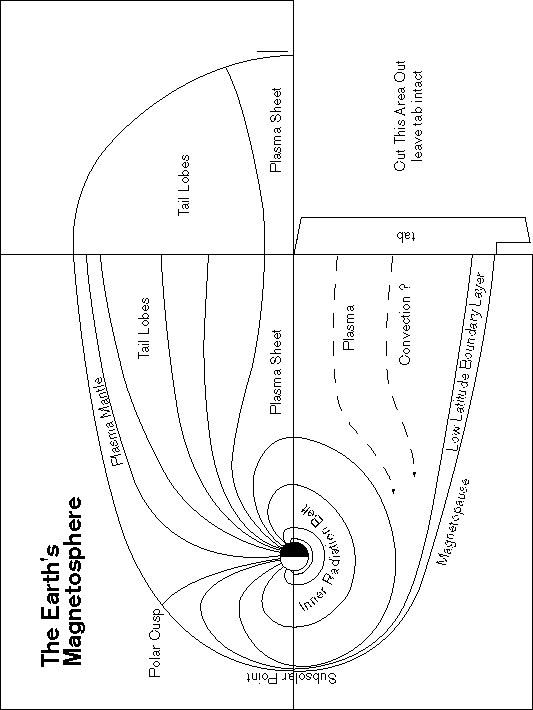
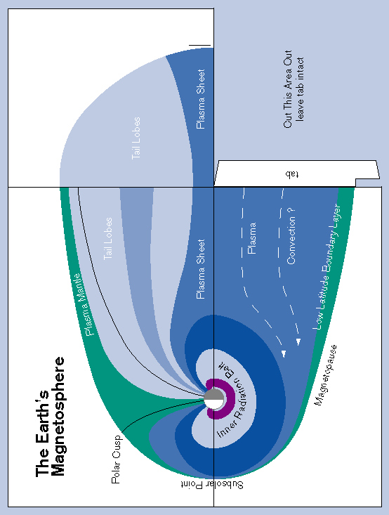
Below are instructions for making a simple paper model of the magnetosphere, out of a single sheet of paper. Read the instructions below first, then link to an image of the model. Print the image, then fold the printout or a xerox copy of it (preferably, one copied onto thick "construction" paper) according to the instructions. Click here to link one of two images, in black and white or in color. The black and white image can be copied in an ordinary xerox machine and can be colored by you in whichever way you prefer. However, if you have a color printer, especially one that can handle construction paper, you might want the second version. Either version is printed out lengthwise, like an ordinary sheet of text.
Instructions
|
|
Much could be learned about space if only it were possible to suspend a satellite motionless in space, observing changes of magnetic fields and particle flows at one fixed spot. It cannot be done. To stay up and resist gravity, a satellite must be constantly on the move and must follow its prescribed orbit. The best we can do is station-keeping: for instance, the motion of a satellite in a synchronous orbit around the equator is matched by the rotation of the Earth below it, allowing it to permanently stay above the same equatorial spot.
Station-keeping in orbits around the SunWith enough velocity, a spacecraft can break loose from the Earth's gravity and enter an orbit around the Sun, like that of a planet. If it then orbits the Sun with the same period as the Earth--one year--it may keep a fixed position relative to Earth. In particular, if that position is between the Sun and the Earth, the spacecraft can be an "early warning station", intercepting any changes in the solar wind before they reach Earth.However, orbital laws require planets closer to the Sun to move faster, by a formula found in 1619 by Johannes Kepler. While the Earth goes around the Sun in 365 days, Venus which is closer only needs 225 days and Mercury, closer still, only 88. Thus any spacecraft going around the Sun in an orbit smaller than the Earth's will soon overtake it and move away, and will not keep a fixed station relative to Earth.
|
|
However, there is a loophole. If the spacecraft is placed between Sun and Earth, the Earth's gravity pulls it in the opposite direction and cancels some of the pull of the Sun. With a weaker pull towards the Sun, the spacecraft then needs less speed to maintain its orbit.
|
If the distance is just right--about 4 times the distance to the Moon or 1/100 the distance to the Sun--the spacecraft, too, will need just one year to go around the Sun, and will keep its position between the Sun and the Earth. That position is the Lagrangian Point L1, so called after the French mathematician who pointed it out, Joseph Louis Lagrange (1736-1813).
|
|
The sister-site From Stargazers to Starships discusses Lagrangian points in more detail than is done here, among other things deriving the distance of L1 (the derivation of L2 is almost identical) and also the equilibrium points L4 and L5. While neither calculation requires calculus, both are somewhat lengthy and assume familiarity with basic principles of Newtonian mechanics, covered in preceding sections of the "Stargazers" site.
|
Spacecraft Observatories at L1The L1 point is a very good position for monitoring the solar wind, which reaches it about one hour before reaching Earth. In 1978 the "International Sun-Earth Explorer-3" (ISEE-3) was launched towards L1, where it conducted such observations for several years. Equipped with an on-board rocket and an ample supply of fuel, ISEE-3 was later moved to the Earth's distant tail and still later was sent to intercept Comet Giacobini-Zinner. In November 1994 a new spacecraft, "WIND" was launched towards that position. It was originally scheduled to be stationed by 1996 in an orbit about the L1 point, but later it was sent on a more extended mission in a "flower petal" orbit around Earth. More recently the solar wind at L1 has been monitored by the solar observatory "SOHO" and by "ACE" whose main task is the study of energetic particles accelerated near the Sun.Such a spacecraft must have its own rocket engine. First, the position is unstable: if the spacecraft slips off it, it will slowly drift away, and sooner or later some correcting action is needed. In fact, the preferred position is actually some distance to the side of L1, for if the spacecraft is right on the Sun-Earth line, the antennas which track it from Earth are also aimed at the Sun, a source of interfering radio waves. Thus corrections are in fact needed quite regularly. Furthermore, the most economic way of getting to L1 is letting the spacecraft pass close to the Moon and using the moon's gravity to extract an extra boost from the Moon's orbital motion. Those maneuvers too require on-board propulsion, as does the final approach to L1.
Other Lagrangian PointsThere exists another Lagrangian point L2 at about the same distance from Earth but on the night side, away from the Sun. A spacecraft placed there is more distant from the Sun and therefore should orbit it more slowly than the Earth; but the extra pull of the Earth adds up to the Sun's pull, and this allows the spacecraft to move faster and keep up with the Earth. The L2 point has been chosen by NASA as the future site of a large infra-red observatory, the Next Generation Space Telescope.
|
| There exist altogether 5 Lagrangian points in the Sun-Earth system and such points also exist in the Earth-Moon system. Among these, the most attention has been given to the two stable points L4 and L5, located in the Moon's orbit but off the position of the Moon (see picture). These positions have been studied as possible sites for artificial space colonies in some (very!) distant future.
|
For those interested in space colonies at the Lagrangian points:
|
Next Stop: #22. The "Wind" Spacecraft
-------------------------------------------------
|
That plan was later changed (see further below) when the solar observatory SOHO was placed in a similar orbit. "Wind" was then moved to a complicated orbit which allows it to sample different parts of space around Earth, while continuing to observe the solar wind. It still carries a large reserve of fuel for its rocket engine.
|
|
ISTP also includes NASA's Polar
spacecraft (launched 24 February 1996), Japan's Geotail (1992) and SOHO
(1995);
other spacecraft will also be involved in ISTP research, including Russia's Interball (1995). The ISTP
effort cuts across
national boundaries. Two US-supplied intruments ride on Geotail; a French
instrument and the
first-ever Russian instrument to fly on a US spacecraft are both part of the
Wind complement of
instruments. Scientists all over the world plan are sharing ISTP data and
collaborating in its
analysis, often with the help of the World Wide Web.
Encounters with the Moon |
| The original plan called for "Wind" to approach its final station over two
years, undergoing two close encounters with the Moon to boost its speed. A spacecraft approaching a stationary
object--like a comet approaching the Sun--increases its speed as it approaches, but after it passes (assuming there has been no collision) it loses again all it had gained.
If however the object is moving, the encounter is not symmetric, and in the end the spacecraft may have gained or lost speed, depending on its trajectory. The encounters of the space probes Voyager 1 and 2 with Jupiter not only helped them explore that giant planet and its magnetosphere, they also gave the Voyagers an extra boost which allowed them to continue to Saturn, where another boost helped Voyager 2 continue to Uranus, Neptune and beyond. "Wind" used the Moon's gravity in a similar manner, as did Geotail.
|
Instruments and ObservationsSome of the instruments aboard Wind measure properties of the solar wind plasma--for instance, the speed of its flow, the flow's direction (it can vary by a few degrees) and the distribution of electron and ion energies. They also measure the proportions of various ions in the solar wind: protons and alpha-particles form the great majority, but the stream also includes the rarer isotopes of "heavy" hydrogen and "light" helium, as well as carbon, oxygen and other elements. The variation of these proportions can shed light on processes in the Sun's corona, where the solar wind originates.Radio wave receivers monitor emissions from the Sun and from space plasmas, and a magnetometer samples the interplanetary magnetic field (IMF) up to 44 times a second. Because the IMF is very weak (about 1/10,000 the Earth's surface field), the magnetic fields produced by electric currents on the spacecraft are strong enough to disturb its observation, and the magnetometer is therefore placed (here and on most deep-space spacecraft) at the end of a long boom, away from the interference. "Wind" also carries two gamma ray detectors, to observe and time gamma ray bursts from distant space, probably beyond our galaxy (more on them in the section on high energy particles in the universe
Dateline December 1998At the end of 1997, WIND rounded the L1 Lagrangian point and headed back to Earth. With the ACE spacecraft now positioned near L1, capable of routine monitoring of the solar wind, WIND with its unique capabilities can be positioned elsewhere, providing broader coverage of the solar wind as we approach the next sunspot maximum, around 2000-2001. The new set of orbits is achieved by flying near the moon and using its gravity to alter the spacecraft trajectory. As of the end of 1998, the new mission is well under way, with "WIND" in its new "petal orbits" which explore the magnetosheath at points abreast of the magnetosphere but relatively distant from the ecliptic. For additional details and updates, see the home page of the "Wind" mission.
|
Next Stop: #23. The Tail of the Magnetosphere
|
In contrast to the dayside magnetosphere, compressed and confined by the solar wind, the nightside is stretched out into a long "magnetotail". This part of the magnetosphere is quite dynamic, large changes can take place there and ions and electrons are often energized.
|
|
|
|
| Solar wind near Earth | 6 ions/cubic centimeter |
| Dayside outer magnetosphere | 1 ion/cubic centimeter |
| "Plasma sheet" separating tail lobes | 0.3 -- 0.5 ions/cubic centimeter |
| Tail lobes | 0.01 ion/cubic centimeter |
|
This extremely low density suggests that field lines of the lobe ultimately connect to the solar wind, somewhere far downstream from Earth. Ions and electrons then can easily flow away along lobe field lines, until they are swept up by the solar wind; but very, very few solar wind ions can oppose the wind's general flow and head upstream, towards Earth. With such a one-way traffic, rather little plasma remains in the lobes.
|
|
We have already met two systems of electric currents in the magnetosphere--the ring current carried by trapped plasma, and the magnetopause current confining the magnetosphere to the inside of a cavity in the solar wind, a current that flows on the surface of that cavity. A third system is the cross-tail current flowing across the plasma sheet from dawn to dusk (drawing below).
| 
|
| It is easy to see that the tail must contain additional currents, for the stretching-out of the tail lobes amounts to adding a magnetic field to the magnetosphere. Any magnetic field in space requires some electric current to produce it, and the cross-tail current can be viewed as the source of the tail lobes. Like every steady electric current, it too must flow in a closed circuit, and the closing occurs in two branches that follow the magnetopause around either tail. |
|
Because of the weak field in the plasma sheet, the ions and electrons of the plasma sheet are constantly stirred up, and some of them--especially electrons--continually leak out of the ends of their magnetic field lines. As such electrons approach the Earth, most bounce back thanks to the action of converging field lines (see the section on trapped particles), but some reach the atmosphere and are lost, producing in the process a diffuse aurora. The eye usually cannot see this spread-out glow, but satellite cameras do so quite well, showing a "ring of fire" surrounding the Earth's polar caps at most time, like the one picturedbelow.
| 
|
|
The diffuse aurora was discovered by the Canadian spacecraft ISIS 2 in 1972, and it expands and contracts as the tail lobes swell and shrink due to variations in the solar wind and its magnetic field. It was extensively observed by (among others) the US Dynamics Explorer mission (1981-7), more recently by the Swedish satellites Viking (1986) and Freja (1992), and currently by the ISTP observatory on "Polar" .
James Dungey's theory of reconnection suggested an answer of sorts. Recall (section on the magnetopause) that in an ideal plasma, ions and electrons that share a field line move together and continue sharing it at all times ("like beads on a wire"). Dungey pointed out an exception to this rule, that when the plasma flowed through a "neutral point" or "neutral line" at which the magnetic force was zero, the plasmas on both sides of that point could become separated and could "reconnect" to different field lines.
|
| Dungey suggested that such a neutral point existed near the front of the magnetopause (marked N on the drawing). He proposed that interplanetary field lines (with the plasma riding on them) linked up there with terrestrial ones, forming compound lines like the one to the right of "3" in the drawing. |
|
That line contains a sharp bend: most of the plasma on the section beyond the bend is interplanetary, most of it on the section closer to Earth is terrestrial. However, both plasmas move together, continue to share the same line, and slowly intermix. A while later, that line would have moved to position of the line right of "4", then to the position "5", and after that, perhaps half an hour later, the reconnection process would be reversed somewhere downstream of Earth, at a neutral point or line near the number "6". The interplanetary parts are then rejoined and flow away, and the terrestrial halves are reunited too. Neglecting spill-over at boundary points like the sharp bend in line "3" (and glossing over some important, and as yet not completely understood, plasma physics), one realizes that the above process will transport near-noon plasma, originally earthward of the bend on line "3", to the distant tail. Dungey proposed that the plasma then flowed back earthward, through the plasma sheet.
|
|
This would create a steady circulation of plasma in the magnetosphere and would also bring fresh ions and electrons into the plasma sheet, from the vicinity of "6". The process is often named "convection", a name used for circulating flows produced by heat, for instance the flow of water in a heated pot (drawing).
| 
|
|
At this point one should look again at the line-sharing property. If all particles on a field line move together, as tail plasma convects back earthward, the particles on the same field lines but just above the atmosphere must keep up with it. Flows of plasma in that region, consistent with Dungey's prediction, have indeed been observed by probing antennas and by "driftmeter" instruments aboard near-Earth satellites, in orbits that cross the polar regions at low altitudes. The electric field associated with them has also been measured, and for that reason most scientists now support the notion of circulating plasma. However, in the tail itself the earthward flow has been harder to confirm and seems to be rather irregular, coming in fits and bursts, especially during magnetic substorms. The distant neutral point near "6" is hard to pinpoint using only isolated satellites, and other plasma processes may also play a help break the temporary links between terrestrial field lines (with their plasma) and interplanetary space. "Geotail" observations suggest that this separation occurs about 70-100 RE away on the night side
|
Next Stop: #24. Substorms
|
The Earth's magnetosphere, like the Earth's atmosphere, is never at rest. Of its many dynamic features, perhaps the most important and basic is the so-called magnetospheric substorm, a period of the order of one hour or less, during which energy is rapidly released in the magnetospheric tail. During substorms, in the polar regions, aurora becomes widespread and intense, also much more agitated, and the Earth's magnetic field is disturbed. Out in space, ions and electrons flow in much greater numbers and at higher energies, and changes in the magnetic field are much more profound than those seen at Earth.
Substorms and Magnetic StormsIn the 19th century and the first half of the 20th, the magnetic disturbances which received the greatest attention were "magnetic storms", so named by Alexander Von Humboldt. These decreases in the magnetic field are world-wide and are readily observed at any place. Typically, a storm takes about half a day to develop, and it gradually decays over the next few days.Magnetic storms are relatively rare. On the other hand, smaller "substorms" observable mainly in polar regions (and in space!) present a clearer pattern and seem to be more fundamental. They are also much more frequent, often just hours apart. The two are of course related, and during magnetic storms intense substorms are generally observed in the polar regions. "Storms" distinguish themselves by injecting appreciable numbers of ions and electrons from the tail into the outer radiation belt, and their world-wide magnetic disturbance reflects a rapid growth of the ring current. Substorms usually do not inject as many particles. It might thus be that magnetic storms are merely sequences of very intense substorms, but additional factors are also involved--in particular, magnetic storms require external stimuli such as the arrival of a shock front or a fast stream in the solar wind.
Substorms at Earth and in SpaceOn Earth the most visible sign of a substorm is a great increase of polar auroras in the midnight auroral zone. At ordinary times, quiescent auroral arcs are often seen there, but following the onset of a substorm, they intensify, move rapidly (mostly poleward) and expand, until they may cover much of the sky. Their activity may build up for half an hour and then decay, but as with atmospheric weather, patterns are quite variable.Large magnetic disturbances are also observed, up to 1000 nT (nanotesla) which is about 2% of the total field in the auroral zone. The world-wide disturbance observed in a magnetic storm of respectable size may only reach 100 nT, but then, its source is much more distant, namely, the ring current which circles the Earth at distances of tens of thousands of kilometers. The electric currents associated with the substorm, on the other hand, come down to the ionosphere, only about 130 km above the ground.
|
|
(above) The record of electrons intercepted by the synchronous satellite ATS 6 on 20 July 1974. The jagged peaks mark the arrival of electrons in substorms, and they gradually drift away again. The lower energies which persist belong to the plasma sheet in which the satellite is immersed for about half of its orbit.
|
|
Much more profound changes are observed in space. Satellites in synchronous orbit which find themselves near midnight when a substorm erupts may see the magnetic field drop by half, and their on-board detectors in general register the arrival of many ions and electrons with (typically) 5-50 keV. These particles can affect a spacecraft, and in particular, the electrons may charge it negatively to hundreds and even thousands of volts, which could interfere with normal operations. With over 200 communication satellites inhabiting the synchronous orbit, there is obviously a good reason for studying substorm effects there. Still further out, in the plasma sheet, very fast flows of plasma are often seen, typically at 100-1000 km/sec; the plasma particles also seem to have higher energies than normal, and magnetic fields change rapidly and erratically. It is not easy to piece together a pattern from such observations, since most of the evidence comes from isolated satellites. What seems to happen is that magnetic field lines of the tail are first stretched tailwards and are then released, in a way frequently compared to the stretching and rebounding of a slingshot. As the lines bounce back, they propel and energize ions and electrons in the midnight region, at typical distances of 6-15 RE.
Substorm EnergyMost natural phenomena require an input of energy, which is then changed to some other form. This also holds true for substorms. It seems no accident that they generally occur when the interplanetary magnetic field (IMF) has a southward slant, which as noted in the discusion of the open magnetosphere, is a time when interplanetary field lines might be more strongly linked to those of the Earth and more energy flows from the solar wind to the magnetosphere.
|
| This is also (as noted there) a time of faster "reconnection" between interplanetary and terrestrial field lines, a time of more rapid "peeling away" of magnetic field lines from the day side (together with their attached plasma), as they become attached to interplanetary field lines and are dragged with them into the tail. Any over-all plot of magnetospheric field lines shows the lines parted like combed hair: one group closes on the day side, around noon, another group is pulled back into the tail lobes, and the cusp marks the groups' separation. Increased "peeling away" near noon shifts the balance: fewer lines go sunward, more into the tail, and the cusp shifts to a field line anchored closer to the Earth's equator. Such a shift leads to two effects.
| 
|
|
First, it weakens the Earth's magnetic field near noon, where plasma and field lines have been peeled off, allowing the solar wind to push its way closer to Earth. As a result, when the interplanetary magnetic field (IMF) is "southward", the "nose" of the magnetosphere is seen to be (on the average) about 1 RE further earthwards than with "northward" IMF, out of a mean distance of 10-11 RE. Secondly, more of the magnetic field is drawn into the tail, and the tail lobes expand, storing additional magnetic energy in them. It is widely believed that the expanded lobes are the main storehouse of energy which powers the substorm. Sometimes, in "clean" substorms when the IMF suddenly "turns southward" after a long quiet period, one can observe this reservoir of energy charging up, as the tail field intensifies and magnetic field lines in synchronous orbit become increasingly stretched tailwards, slingshot-like. This "growth phase" typically lasts 40 minutes. |
|
The exact way in which this energy is released, and the "trigger" which starts the process, are still subjects of debate and controversy. But it is widely held that the critical event is the formation of an X-shaped neutral point, or more likely, a neutral line extending some distance across the tail. That is not the distant neutral point of Dungey's theory, but an additional one formed quite close to Earth, at a distance of 15 to 30 RE (drawing on right).
| 
|
|
Magnetic reconnection then begins between oppositely directed field lines north and south of the middle of the plasma sheet (the "equatorial plane"), as explained in connection with the open magnetosphere. Each line on the northern side is broken in two at the neutral line, and the parts are spliced to corresponding parts of a line from the southern side, which is similarly divided in two. The broken and reconnected halves of lobe field lines form two new lines. The one on the earthward side, essentially a stretched terrestrial line, rebounds earthward, just like a released slingshot. The other one is connected tailwards, and because it no longer has any connection to Earth, it is expelled down the tail. Together with the plasma riding on it (and other plasma, originally further tailwards), it forms a sort of a plasma bubble known as a "plasmoid" (see drawing above). The passage of such plasmoids further down the tail has been deduced from observations by ISEE-3 and Geotail. Initially the newly-reconnected lines are those of the plasma sheet, but as the process sucks in magnetic field lines from both sides towards the neutral line, the tail lobes are soon reached. The effect on the magnetic field piled up in the lobes, and on the energy stored in them, is somewhat like that of a pin on a well-inflated balloon. Just as the pinhole allows air to escape and releases the energy stored in the balloon, so the neutral line allows field lines (with their plasma) to leave the lobe, reducing both the intensity and energy of the magnetic field there. Energy in nature is conserved. If it disappears in one form, it reappears in another: electric energy consumed by a motor is converted to kinetic energy of motion, and when motion is stopped by friction, its kinetic energy turns to heat. The magnetic energy taken from the tail lobes also reappears in different forms. Some is turned to heat, that is, it raises the velocity and hence the energy of plasma ions and electrons (heat being the kinetic energy of individual particles moving in disordered fashion--in both a gas and a plasma). The plasma most likely to be heated in this process is the one attached to the reconnected field lines: since those lines come from the tail lobes, whose plasma is extremely rarefied (see magnetotail), rather few particles share this energy and therefore the amount each of them receives may be quite big.
Electric CurrentsSome of the converted energy ends up driving electric currents, in a circuit linking the plasma sheet and Earth. The connecting links are magnetic field lines, which can conduct electric currents quite well, since ions and electrons attached to field lines slide rather easily along them.
|
|
As noted (section on magnetotail, also drawing on right), a large electric current flows at all times across the plasma sheet, from the dawn edge to the evening edge (and then closes along the magnetospheric boundary). In a substorm some of this current, it seems, is diverted earthwards along magnetic field lines.
|
|
|
The diversion starts in the morning-side half of the plasma sheet, where currents are withdrawn to flow earthward along field lines. They then continue (mostly) in the ionosphere, and finally return to space along other field lines, to the evening-side of the tail. The by-passed section in the middle of the plasma sheet, where the cross-tail current is weakened, seems also to be the region actively involved in the substorm, but how the substorm disrupts there the orderly flow of the cross-tail current is still a matter of controversy. The flow of electric currents along field lines may also be the key to the production of the substorm aurora, as will be discussed later.
Substorms in PerspectiveThe preceding account is explicit and tidy, suggesting a rather clear picture of what goes on in a substorm. Actually, much is guesswork: we have some pretty reasonable hunches, but nature may yet surprise us. For instance, the details of reconnection in the tail are hard to confirm, and its location and even existence are still being disputed.Even though the physics is quite different, one can compare a substorm to a thunderstorm. Meteorology experts have a clear and orderly view of this phenomenon: its energy is supplied by the moisture contained in warm, humid air, and a rising flow forms an updraft (like the rising central column in the pot shown in the section on convection), extending to great heights. One can describe the processes controlling the flow of air in that central "updraft" and the formation of rain (and even of lightning, a somewhat peripheral phenomenon). But a look at an actual thunderstorm reveals no tidy structure: flows are obscured by clouds, patterns are deformed, neighboring thunderstorms affect each other, and each storm is in fact different. An observer watching from the ground may find it hard to draw any conclusions. Launching balloons with instruments into the storm could help, but if only a few are available, their evidence may be contradictory, since those that miss the rising updraft move unpredictably. Substorms are like that, too, only more difficult--because of their greater distance and size, the small number of satellites available and perhaps the greater intricacy of plasma phenomena. Almost all we know about them comes from ground observations or from isolated satellite passes, which cannot be readily combined, since each storm behaves differently.
|
Next Stop: #25. Electric Currents from Space
|
When a bright aurora is seen in the auroral zone, a strong magnetic disturbance is usually also observed there. The disturbing magnetic field can be much stronger than that of a magnetic storm but it is strictly local, fading away quickly as one moves equatorward. This limited extent suggested that the currents which disturbed the field flowed somewhere nearby, probably near the auroral arcs. The Norwegian Kristian Birkeland, who carefully observed auroral disturbances around the turn of the century, concluded that those currents flowed parallel to the ground, along the auroral formation.
|
| Any electric current, however, must flow in a closed
circuit, and since it seemed to be caused (like that of the aurora) by processes taking place in distant space, Birkeland proposed that it came down from space at one end of the arc and returned to space at the other end. The drawing below illustrates the idea and was taken from Birkeland's 1903 report on his
expeditions to the auroral zone:
|
|
|
|
The idea was sound, but the current was too weak to be measured by him.
Faraday nevertheless speculated that the aurora (which he believed to be an
electric phenomenon) might be powered in a similar way by the Gulf Stream
flowing to the north-east through the Atlantic Ocean, beginning just offshore
from the US. Of course, what Faraday forgot here was that to connect the ocean to the aurora, the current would have to cross the lower atmosphere, which is an excellent insulator and would block its flow. An interesting dynamo of this type exists between the planet Jupiter and its innermost big moon Io (click for details). The space shuttle can also generate electric power that way (at the expense of its orbital energy), using a long wire dangling from it into space. Such a space tether experiment was conducted aboard the space shuttle Columbia on 25 February, 1996, ending unexpectedly when the tether suddenly broke. Sir Joseph Larmor in England first proposed in 1919 that dynamos consisting entirely of fluids might explain the creation of sunspot magnetic fields. His idea was that as solar plasma flowed through magnetic fields, dynamo effects produced the very same currents which also created those magnetic fields. Because this is a process which "lifts itself by its own bootstraps" (the magnetic fields needed by the dynamo are produced by the electric currents which are its output), it must build up gradually, starting from some "seed" magnetic field of a different source. Such a "dynamo mechanism" was also believed to be the source of the magnetic field arising inside the Earth's molten core. It is impossible to observe that region directly, but in 1964 Stanislaw Braginsky, in Russia, mathematically demonstrated a possible class of such "dynamos." The slow decade-by-decade variation of the Earth's field probably comes from slow changes in the flow patterns of the core - not, as Halley once proposed, from magnetized spherical layers, one inside the other, all rotating differently.
If the bundle of open lines maps to the region inside the auroral oval, it can be shown that the "dynamo currents" from the above process flow earthward on the morning side of the magnetic pole and spaceward on the evening side. One might guess that the circuit would be completed by connecting the two flows across the polar ionosphere, from the morning side, to the evening side (drawing below; the situation is more complicated, however, because the flow also deforms the field lines).
|
|
|
|
But that wasn't all. Equatorward of each current sheet, Triad noted a
parallel sheet almost as intense, flowing in the opposite direction: those field lines were no longer open, but closed inside the magnetosphere. It thus seemed that most of the electric current coming down from space (about 80%) did not choose to close through the ionosphere across the magnetic poles. Rather, it found an alternate way: it flowed in the ionosphere a few hundred miles equatorward and then headed out again to space, where the currents (presumably) found an easier path.
|
|
A 1976 study by Takesi Iijima and Tom Potemra used Triad data to map the
average "footprints" of these sheets in the polar ionosphere, including their
intricate overlap at midnight. Their result is plotted below: the map is centered at the northern magnetic pole (though southern data were combined to produce this graph), midnight is at the bottom, and noon (where some minor additional currents exist) is at the top. Dark shading indicates currents flowing towards Earth, light shading, currents flowing outward into space.
| 
|
Next Stop: #25A. Currents from Space--History
|
As noted earlier Kristian Birkeland, reporting in 1903 on his expeditions to
the auroral zone, proposed that magnetic disturbances accompanying the aurora were caused by large electric currents flowing down the length of auroral formations. These formations generally follow the contours of the auroral zone, and Birkeland felt that the current entered them at one end and left at the other.
|
|
|
In later years these currents became known as the auroral electrojets, and considerable debate ranged over their cause and the way their circuit might be completed. Some scientists disagreed with Birkeland and claimed the electrojets did not connect to space but instead their entire circuit lay inside the ionosphere, like that of other ionospheric currents known at the time, believed to be caused by atmospheric tides. In 1969 Schield, Dessler and Freeman, supporters of Birkeland's ideas, proposed a fairly detailed theory of how such currents might originate in space, and also predicted the secondary "region 2" currents. They even proposed a name for them--"Birkeland currents." That same year Naoshi Fukushima in Japan pointed out that such "Birkeland currents" connected to the ionosphere would be almost "invisible" from the ground, producing there only a very weak magnetic disturbance, because magnetic fields contributed by various parts of their circuit tended to cancel out.
|
| And that was actually the case. When the large-scale pattern of such currents was finally recognized, in 1973, they were found to flow mainly in two parallel sheets, connected across the electrojets rather than along them. |
|
The drawing above shows narrow sections of these sheets on the morning and evening side, viewed from midnight, with the current closing around midnight as drawn; only narrow sections are shown, because one cannot draw the full sheets without having them obscure each other. The flow of current is in alphabetical order, from A to B .... to G As Fukushima had foreseen, that circuit had only a small effect on magnetometers on the ground.Instead, the disturbances measured at the surface of the Earth come mainly from the electrojets, which are a by-product of the main circuit due to the unusual electric conductivity properties of the ionosphere. It is possible that they indeed close largely in the ionosphere. Although signs of currents flowing from space along magnetic field lines were occasionally detected by earlier satellites, it was the US Navy's Triad, carrying the instrument of Alfred Zmuda and James Armstrong, that in 1973 traced their full pattern. Triad was an experimental navigation satellite, and it circled the Earth in a low altitude orbit which went from pole to pole, while the Earth rotated beneath it. Zmuda and Armstrong were allowed to place on it a magnetometer as an extra "piggyback experiment," and it continued to return scientific data for many years after the Navy's experiment had ended. When Triad crossed a current sheet, a characteristic "signature" was generally noted: the direction of the magnetic field rotated fairly abruptly, while its strength stayed practically the same. From such rotations a wealth of information was extracted about the structure and variation of the currents. Tragically, both experimenters had died by the time their article on "Birkeland currents" appeared in 1974.
|
Next Stop: #26. The Polar Caps
|
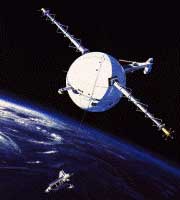
Triad, launched September 2, 1972, was an experimental spacecraft designed to
move in an accurately predictable low-altitude orbit, allowing its position to
be used as a reference point in navigation.
|
 The Triad Spacraft.
|
|
|
While the "proof mass" thus moved in an accurately predictable orbit, the
spacecraft itself was subject to air resistance and sunlight pressure, causing
it to move slightly differently. Electronic sensors would note when the
floating ball approached one of the walls of its "cage", and thrustors would be
fired to move the spacecraft away from the ball. By thus matching its motion to
that of the "proof mass", the satellite moved as if no extra disturbing forces
existed. It worked until the spacecraft ran out of fuel. However, it was tracked for many years afterwards because of the value of its magnetometer observations.
|
|
The giant planet Jupiter has four large moons, discovered by Galileo and
visible through good binoculars. It has in addition many smaller ones, as well
as a narrow ring like Saturn's, observed by the spacecraft Pioneer 11. Of the large moons--comparable to our own moon or bigger--the outer three are icy spheres, but the innermost one, Io, is heated by tides, and as a result has volcanoes and an ionosphere which is a fair conductor of electricity. Jupiter itself like Earth is a magnet, but one that is 20,000 times stronger; as a result it has a large magnetosphere and a very intense radiation belt. A dynamo is created in a magnetic field by an electric circuit, part of which is moving relative to the rest (additional conditions must also be met). The circuit may consist entirely of fluids (as in sunspots), but solid conductors can also be involved.
|
|
The conditions for a dynamo are fulfilled in the case of Io and and Jupiter.
Both are conductors, and they move quite differently--Io orbits, Jupiter
rotates. Furthermore, the plasma between them conducts electricity very well
along its magnetic field lines, which act as if they were wires connecting Io
and the planet (drawing). One expects a continuous current to flow in this
circuit, feeding on Io's orbital energy.
| 
|
|
The drawing is not to scale. Actually Io is much smaller. Watchful readers may notice that the north-south magnetic polarity of Jupiter is the reverse of what it is for Earth. They might also note that if the drawing views Jupiter from the Sun's side, Io actually orbits in a direction opposite to that of the arrow. However, the plasma which fills space around it rotates with Jupiter and moves much faster, overtaking Io. Relative to the plasma, therefore, Io moves backwards. The path of the space probe Voyager 1 was designed to check out this dynamo, by flying close to where its currents were expected to flow. It did so on March 5, 1979, and its magnetometer very clearly detected the signature of a current of about a million amperes. Previous to that it was noted that unlike any other moon of Jupiter, Io had a strong influence on radio emissions from Jupiter's magnetosphere, which depended on its position: it could be that the moon's unique electric currents were involved in this.
PostscriptsThe Hubble Space Telescope, using its Wide Field and Planetary Camera 2, has been photographing auroras of the planet Jupiter. Recent pictures,taken in ultra-violet light, have shown not only rings of aurora around Jupiter's magnetic poles, but also a spot of light, formed where the magnetic field lines of Io reached the surface. Presumably, they represent a special kind of aurora, powered by the electric currents of the Io dynamo. A recent picture shows not only the footprint aurora of Io (which also leaves an auroral "trail" behind it), but also spots of light attributed to auroras formed in a similar manner by Europa and Ganymede, more distant moons of Jupiter.See here for a picture of Io "in its true colors" and links to sites about it.
|
|
The space tether experiment, a joint venture of the US and Italy, called for
a scientific payload--a large, spherical satellite--to be deployed from the US space shuttle at the end of a
conducting cable (tether) 20 km (12.5 miles) long. The idea was to let the
shuttle drag the tether across the Earth's magnetic field, producing one part of
a dynamo circuit. The return current, from the shuttle to the payload, would
flow in the Earth's ionosphere, which also conducted electricity, even though
not as well as the wire.
| 
|
|
One purpose of such a set-up might be to produce electric power, generating
current to run equipment aboard the space shuttle. That electric comes at a price: it is taken away from the motion energy ("kinetic energy") of the
shuttle, since the magnetic force on the tether opposes the motion and slows it down. In principle, it should also be possible to reverse this process: a future space station could use solar cells to produce an electric current, which would be pumped into the tether in the opposite direction, so that the magnetic force
would boost the orbital motion and would raise the orbit to a higher
altitude. An earlier tether experiment ended prematurely when problems arose with the deploying mechanism, but the one on February 25, 1996, began as planned, unrolling mile after mile of tether while the observed dynamo current grew at the predicted rate. The deployment was almost complete when the unexpected happened: the tether suddenly broke and its end whipped away into space in great wavy wiggles. The satellite payload at the far end of the tether remained linked by radio and was tracked for a while, but the tether experiment itself was over. It took a considerable amount of detective work to figure out what had happened. Back on Earth the frayed end of the tether aboard the space shuttle was examined, and pieces of the cable were tested in a vacuum chamber. The nature of the break suggested it was not caused by excessive tension, but rather that an electric current had melted the tether. The electric conductor of the tether was a copper braid wound around a nylon string. It was encased in teflon-like insulation, with an outer cover of kevlar, a tough plastic also used in bullet-proof vests, all this inside a nylon sheath. The culprit turned out to be the innermost core, made of a porous material which, during its manufacture, trapped many bubbles of air, at atmospheric pressure. Later vacuum-chamber experiments suggested that the unwinding of the reel uncovered pinholes in the insulation. That in itself would not have caused a major problem, because the ionosphere around the tether, under normal circumstance, was too rarefied to divert much of the current. However, the air trapped in the insulation changed that. As it bubbled out of the pinholes, the high voltage ("electric pressure") of the nearby tether, about 3500 volts, converted it into a plasma (in a way similar to the ignition of a fluorescent tube), a relatively dense one and therefore a much better conductor of electricity. The instruments aboard the tether satelite showed that this plasma diverted through the pinhole about 1 ampere, a current comparable to that of a 100-watt bulb (but at 3500 volts!), to the metal of the shuttle and from there to the ionospheric return circuit. That current was enough to melt the cable. As the broken end whipped away from the shuttle, the plasma established electric contact with the ionosphere directly. The satellite on the distant end monitored the current: after about half a minute it stopped, then it reignited and flowed again for about another half minute, stopping for good when (presumably) all the trapped air was gone. Because of the unexpected break, the tether experiment at the time was widely viewed by the press as an expensive failure. True, the planned operation at full deployment, for several hours, could not take place, nor could the tether and its satellite be retrieved, which was to have demonstrated the feasibility of deployable tethers. However, many of the scientific experiments had already begun during deployment and yielded good data. And the break itself, though unfortunate, added an unscheduled experiment to the mission, one which highlighted the risks and complexities of operating scientific equipment in space.
|
Authors and Curators:
This joined-up file created 10 June 2001