Planning the "Profile" Multiprobe Mission

David P. Stern, Laboratory for Extraterrestrial Physics
Goddard Space Flight Ctr., Greenbelt, MD 20771

Abstract

    The "Profile" mission to the magnetosphere calls for a constellation of 12 satellites in two groups on two nearly identical near-equatorial orbits, extending to 20-25 RE. The satellites in each group would pass apogee about 1 hour apart, they would carry magnetometers and plasma instruments and would spin around an axis perpendicular to the orbit. Thus "Profile" would be able to obtain radial profiles of fields, plasmas and propagating disturbances on a global scale, but it would also cover some small-scale features by its "superclusters" near apogee and its "overtaking" mode of observation.
          This article briefly reviews the results of the "Profile" study since 1996 and its simulations of magnetospheric coverage, data downloading and long-term orbital evolution. It describes

    1.     Design of the mission and its spacecraft
    2.     The "slingshot release" of satellites
    3.     Launch strategies for good plasma sheet coverage without excessive eclipses
    4.    Coverage of various magnetospheric regions and occurence frequency of different "formations."
    5.    Considerations of battery-free operation and of radiation damage
    6.     Strategies for the retrieval of data
    7.     Long-term evolution of the mission and strategies for avoiding early atmospheric re-entry.

Genesis and Concept

Two things inspired "Profile". First, the realization that in the last 15 years, the pace of significant discoveries in magnetospheric physics has declined, and that many long-standing questions remain unresolved [Stern, 1996b]. One reason for this state of affairs seemed to be the delay of a transition from isolated satellites to "networks" of larger numbers [Stern, 1996a, sect. 18, item 2].

The other inspiration came from Comet-Shoemaker-Levy, whose fragments were discovered spread out along an elongated ellipse around Jupiter, ultimately hitting the planet in July 1994. This led to the idea of a string of small satellites similarly spread out on an elongated ellipse around Earth--e.g. orbiting one hour apart in an orbit extending to 20 or 25 RE. What sort of significant observations could such a formation conduct? As it turned out, quite a few.

Other "constellation" missions to probe the global magnetosphere have been proposed and some of them are described elsewhere in this volume. They visualize a 3-dimensional network of satellites (usually with different periods) as providing an "image" of the magnetosphere, each satellite giving a single "pixel." Actually, even a crude image of this sort requires a hundred (if not a thousand) satellites, creating a rather elaborate and expensive mission, whose data are hard to analyze because the relative positions of the satellites constantly change.

Placing all satellites in the same orbit reduces coverage to one dimension, to a near-radial cross-section or profile, which gives the mission its name. However, the geometry is persistent: the same line is monitored for a long time and whenever a satellite leaves its position, another usually replaces it within an hour. Instead of using satellites as pixels, whose pattern is only discerned after the fact, here the geometry is "clean." Specific questions can be targeted, as is described in an accompanying article [Stern, 1998]

Because "Profile" calls for a relatively small number of satellites, its data are easier to download and assimilate. It could therefore be a good beginning for global observations by multi-spacecraft constellations, as well as a testbed for perfecting the analysis and modeling of multipoint data, and a springboard for future SEC missions. Although deployment would require new technology, the satellites themselves follow a conservative design and would only require a moderate extension of the current state of the art.

Mission Design

Mission Design The initial concept called for 12 small spinning spacecraft in an elongated near-equatorial orbit (Figure 1, on the right), with apogee of 20 or 25 RE. Instruments included a magnetometer on a short boom (75 cm) and a half-top-hat combined ion and electron detector. The magnetometer would give magnetic field vectors within 1° and 0.5 nT, while the particle detector´s aperture would cover 14° of the spin angle f and 180° of the orthogonal angle q, so that in a single spin cycle, all 4p steradians of space are covered.

The satellites themselves would be hollow hexagonal boxes with sides of 25 cm and height 40 cm, covered with solar cells. Their instruments would be attached to 3 triangular shelves, set up along the "equators" of the boxes, and they would spin around their axes of symmetry. Those axes would be perpendicular to the ecliptic, causing the Sun to heat all parts of the satellite evenly ("barbecue mode") and also to provide a nearly constant solar power. Furthermore, by comparing fluxes 180° apart in the spin cycle, a sensitive estimate could be made of the components of the bulk velocity v in the spin plane, which would be close to the ecliptic.

Using existing technology, a mass of 17 kg per satellite was estimated. This breaks down to 4 kg. for the frame, 4.7 kg for the solar cells (including a 1mm protective glass cover), 0.5 kg for a small battery; as is explained further, mass is invested in solar cells rather than in batteries for the sake of durability, but other possibilities also exist. Other masses may be 2 kg for transponder, 2 kg instruments, 1 kg for computer, memory and data handling and command unit (for which a chip is being developed), 0.3 kg Sun/Moon sensor, 0.5 kg antenna and preamp, and 1 kg wiring and thermal blankets.

Figure 2
One proposed method of carrying

Cross section of the array, which is spun up around its central axis. One pair of satellites is released at each perigee pass.

(2a) One proposed method of carrying "Profile" satellites aboard their mother ship is a hexagonal array.
(2b) Cross section of the array, which is spun up around its central axis. One pair of satellites is released at each perigee pass.

The 12 satellites would be initially attached to a central structure (Figure 2 shows one possible arrangement), aboard a "mother ship" launched into an orbit near the required one. At perigee, one satellite would be ejected forwards in the orbit (or backwards), with a small velocity increment angle Dv, which turns out to be surprisingly small, about 4 m/s. Since that satellite moves into a higher (lower) orbit, its period is longer (shorter) and by the time of the next perigee pass of the mother ship, it lags behind (leads) by one hour. The next satellite is then ejected, and at the following perigee pass by the mother ship, it will lag (lead) by one hour, while the one released earlier lags (leads) by two. And so on, until all satellites are in their new orbits.

A 2-year mission is envisioned, providing two passes through each equatorial region of the magnetosphere. After that the positions of the satellites may shift somewhat, but even then much of the physics can still be carried out. Since such satellites would give valuable synergistic support to any other magnetospheric mission (including other constellations), a design lifetime of 10 years was assumed.

The centrifugal slingshot

Two factors need to be noted. First, all ejected satellites must have precisely the same orbital period, or else they will soon overtake one another. The latter might happen if the releases employ springs, which create recoil, or small rockets, whose delta-v is hard to match exactly. Second, it is difficult to toss a satellite in the direction of the orbital motion while its spin axis remains perpendicular to the orbit; it would have to be a sideways toss, like that of a frisbee.

Both problems are solved by using a "centrifugal slingshot." After entering its elongated orbit, the mother ship is turned by 90° so that its axis (paralleled by the axes of all satellites) is perpendicular to the ecliptic, and it is then spun up around that axis. Each perigee pass after that, on cue from a solar attitude sensor, explosive bolts cut loose a pair of satellites, one of them being flung by the rotational motion forwards and the other backwards. The satellites then retain the angular velocity of their mother ship.

Satellite formations and Science Tasks

The centrifugal slingshot release modifies the mission. Rather than 12 satellites with a 48 or 67 hour period (for 20 or 25 RE apogee), we get 6+6 with periods (47, 49) or (66, 68) hours, and the lower group periodically overtakes the higher one.

Mission modification

    Rather than interfering with the scientific goals, this actually enhances them. When the groups overtake, the satellites form "superclusters" at apogee, with most or all of them inside a narrow range of radial distance r (Figure 3). Such clustering is particularly useful for studies of the region where substorms begin, of the low latitude boundary layer (LLBL) and the bow shock. Also, on the sides of the orbit, pairs of satellites--one from each group--would approach each other and then separate again, allowing one to derive 2-point correlations of the magnetic field B, bulk flow v, plasma density n, energy spectra and other features. This would happen nearly simultaneously at different distances, in the plasma sheet, foreshock or sheath.

At other times the satellites would be spread out radially, making possible the tracking and timing (within 1 sec) of substorm disturbances, dispersion-free injections and bulk flows on the night side, and on the day side of shocks, Alfvenic waves and compressions, and of flux transfer events (FTEs). Other observations would include profiles of Bz and vx in the tail, cross-sections of the ring current at frequent intervals, also boundary waves and the flaring angle of the magnetopause. "Profile" has specifically targeted over 20 such tasks, most of which address well-defined questions, listed and discussed in the accompanying article [Stern, 1998].

Simulations of the "Profile" Mission

The "Profile" constellation mission raises some questions which can only be addressed by simulating it on a computer. They include:

  1. How often (in a typical year) do specific satellite formations cover regions of the magnetosphere in the way required by each specific task?
  2. How long are the longest eclipses?
  3. What is the best strategy for retrieving the data?
  4. How do the orbits evolve over the years?
  5. How does the spacing between satellites change?
The variables at one´s disposal include:

    (a)    The radial distances of apogee and perigee
    (b)   The time of day and date of the launch.
    (c)   The option of first injecting the mother-ship
          into a circular low-altitude parking orbit
          and delaying the firing of the last stage
           by a selected time.
    (d)  The number of ground stations and their
         mode of operation.
Two sets of simulation codes were developed. "Keplerian" codes which assume 2-body dynamics were used in answering questions (1), (2) and (3), while "Perturbation" codes took account of perturbations by the Moon, Sun and the bulge of the Earth´s equator and were used for all questions except (3). Only selected results can be presented here.

As a preliminary excercise, a subroutine was produced which, given a satellite at (x,y,z) and time t, derived the region of the magnetosphere in which it was most likely to be found. A somewhat similar (but more elaborate) code was provided by Mauricio Peredo for the Natl. Space Science Data Center (NSSDC). Ten options were encoded by numbers 0 to 9 and are listed below:

    0 -- Inner MS
    1 -- 1 RE or less from MP, inside it.
    2 -- 1 RE or less from MP, outside it.
    3 -- Magnetosheath.
    4 -- Solar Wind.
    5 -- Tail Lobe.
    6 -- PS, z = ±(2.5 ±0.5 RE)
    7 -- PS, z = ±(2.5 ±0.5 RE)
    8 -- PS, z = ±(2.5 ±0.5 RE)
    9 --Transition, PS to inner MS.
(MP=magnetopause, PS=plasma sheet, MS=magnetosphere).

After the orbital elements and the launch time (or equivalent information) were chosen, a simulated constellation was followed hourly for a "year" of 52 weeks, and track was kept of the total time spent by the satellites in each region. Statistics were also kept, for each of the 52 weeks, of the simultaneous occupancy (9+ meaning " 9 or more") of:

    (a)   Regions (7)+(8) by 1, 2, ... 9+ s/c
    (b)  Regions (1)+(2) by 1, 2, ... 6+ s/c
    (c)   Each of (0), (1)+(2), (3) and (4) by 2+ s/c
    (d)   The region r > R1 by 5, 6, .. 11+ s/c,
         R1 being typically 2 RE short of apogee.
    (e)    Like (4), but with all s/c in the PS.
    (f)   With 3+ s/c at r < R1 on each side of the orbit.
    (g)   A weekly tally of eclipses of 1, 2,... 9+ hours.

Depending on the time of day of the launch--assumed to be eastward from Cape Canaveral, latitude 28.5° N--the orbital inclination ie to the ecliptic can range from (28.5°-23.5°) = 50° to (28.5°+23.5°) = 52°. The best coverage or regions (6)-(8) and of occupancy classifications (1) and (5) occurs with the smallest ie but it is adversely affected by the hinging and warping of the geotail, due to dipole tilt. That is avoided if the mother ship is first launched into a circular parking orbit and is then permitted to coast over an arc of 90° (or 90°+180° N, N=1,2..) before the last stage fires. This "optimal" orbit was used as a reference orbit, to whose parameters further changes were added.

Actually the reference orbit, whose axis lies along the celestial x-axis, is anything but optimal, since it has the longest eclipses--7 hours for 47±1 hour periods, 10 hours for 67±1 hour ones. In general, the coverage of the plasma sheet was found to depend strongly on ie and to correlate with eclipse duration. The best strategy seemed to be to use slightly "detuned" orbits which still gave good PS coverage, with ie around 13° and eclipses of up to 2-3 hours. Long-term perturbations, unfortunately, change ie , bringing (according to circumstances) longer eclipses or worse plasma sheet coverage. Specific choices will have to wait until the mission is better defined.


    Table 1 (below) gives the number of hours per 52-week year spent in each region, for 4 "Profile" missions with two apogee choices and two possible arc lengths in the parking orbit:
    #(1, 2): 47±1 hour period, delay +2 hrs, coasting angle 60° and 110°.
    #(3, 4): same for 67±1 hours.

  0   1   2   3   4
  inner   magnetopause  sheath    SW
#1  14875    6342     5796     18753     18928  
#2  14994    6265     5810     18837     19425  
#3  9933    5271     4942     17563     31703  
#4  9966    5159     4830    17346     32494 

Blocks above and below: Number of satellite-hours spent in various regions of the magnetosphere (listed earlier); 1000 satellite-hrs about equals one percent of the data.

 5    6     7     8     9
 lobe     2.5 RE     1.5 RE     0.5 RE     trans.
#1   21476     7350     4900     4606     826
#2   9548    8050     9002     10892     1092
#3   21182    5481     3934     3549     574
#4   10332    7504     7581     8239     630

Block below: Number of hours (per year) with
    (1) 6+ satell. ±1 RE of magnetopause
    (2) 9+ satell. in plasma sheet (PS) outside apogee,
    (3) 11+ satell.in PS in "supercluster"
    (4) 2 satell. in each of (inner Msphere, mpause ±1RE, sheath, SW)
    (5) duration in hours of longest eclipses and no. of such eclipses.
    In this block, 168 hrs = 1 week.
  6+     9+     11+     2 × 4     eclip.
  #1     708     135     22     174     2 × 12
  #2     631     484     130     201     3 × 71
  #3     635     72      1     156    2 × 12
  #4    488     302     101     172    4 × 16


Eclipses and the Phoenix Mode

Because even 3-hour eclipses cause severe chilling, and because batteries have a limited lifespan, one option of the "Profile" satellites is to adopt a completely battery-free design. It would invest weight in solar panels rather than in batteries, giving the transmitter enough power to download data without recourse to stored energy.

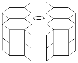
To prevent excessive cooling, thermal blankets would close the top and bottom of the hexagons, keeping the interior above -50° even in long eclipses. A small "keep alive" battery would be placed next to the memory and CPU, keeping them running and in the process generating enough heat to stave off freezing. If that battery fails, the satellite´s computer would automatically enter the "Phoenix mode", go to sleep in eclipses (even short ones near Earth) and start up again afterwards.

The battery would be needed mainly for maintaining the memory: at a data rate of 0.6 to 1 kbit/s, each satellite accumulates about 200 Mbits/orbit, and satellite memories such as the ones now available are "volatile," wiped clean if power is lost. However, the technology of "non-volatile" memories is advancing, and if such memories can meet the needs of the mission, the battery could be omitted without risking data loss, and the "Phoenix mode" could become the main mode of operation.

Radiation and Data Rates

Since the orbit crosses the inner radiation belt, the radiation dosage can be appreciable, especially to exposed solar cells. Even when shielded by a glass cover of 1 mm, these cells may absorb 50 rad/orbit, resulting (at the very least) in a gradual loss of power. To offset this, the initial extra power capacity must exceed needs by about 25%.

As noted, data rates would have to be relatively low, about 0.6-1 Kbit/s (depending on apogee). The data would initially go into a cache containing (e.g.) 5 minutes of detailed data, more than can be transmitted. The cached data would then be pre-screened automatically. If their rate of variation is low (as might happen most of the time), the data would be encoded in a data frame format with low time resolution (e.g. 1 minute) but resolving in detail energy and direction. If on the other hand appreciable variation is encountered, a different data frame might be used, with good time resolution (e.g. 1 sec) but compromising other aspects.

On command from the ground, two alternative data rates would be available, a "low" rate in which only rudimentary data are collected, perhaps 100 bit/sec, allowing a "high" rate (5-10 Kbit/sec) during a limited preselected portion of the orbit. This mode would be employed when orbital calculations predict an interesting coverage by a "supercluster", or other situations when dense data are of interest.

Transmission of Data

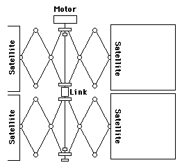
Satellites with spin axes perpendicular to the Sun´s direction, carrying 6 panels of 25 × 40 cm (minus 10% of unusable area), generate on the average 29 watts, which is expected to drop gradually to 22 w due to radiation damage. A conservative estimate then allocates 15 w to the transmitter and assumes 1.5 w antenna power. The antenna is assumed to be omnidirectional, although ways exist of increasing the directional beam strength using a belt antenna or a number of electronically switched antennas with reflectors.

The maximum data rate is then proportional to the area of the tracking antenna and to 1/R2, with R the distance from the tracking station (not the center of the Earth). For instance, a 15-meter antenna would take about 1 hour to download 200 Mbits from R = 5 RE. Such antennas cost about $1,500,000, while a semi-autonomous tracking station can be bought for about $500,000. Antenna costs are approximately proportional to their area, e.g. an 11-meter dish (about 1/2 the area) costs about $750,000 and would need 2 hours for a full download from 5 RE.

The data rate available near apogee is low, but satellites spend most of their time there, making it a-priori unclear which is the best downloading strategy, slowly from far away or rapidly near perigee. It turns out that the latter is by far more advantageous. Two problems then arise:

  1. For a given near-earth pass of a satellite, the rotation of the Earth determines its position relative to any tracking station, and one finds that from most locations on Earth tracking is not practical. That suggests multiple stations, evenly distributed in longitude.
  2. Because satellites of any group follow each other (at least for the first year or two) at 1-hour intervals, downloading should not take more than 50 minutes (plus 10 minutes for switch-over). To make full use of the short time available, satellites should be able to use (say) 5 different downloading modes, each with its own data rate, switching to increasingly faster (slower) modes as the distance to the tracking station decreases (increases). The switching schedule would be updated from time to time by ground command, based on a code like the one described here.

    Simulation of downloading

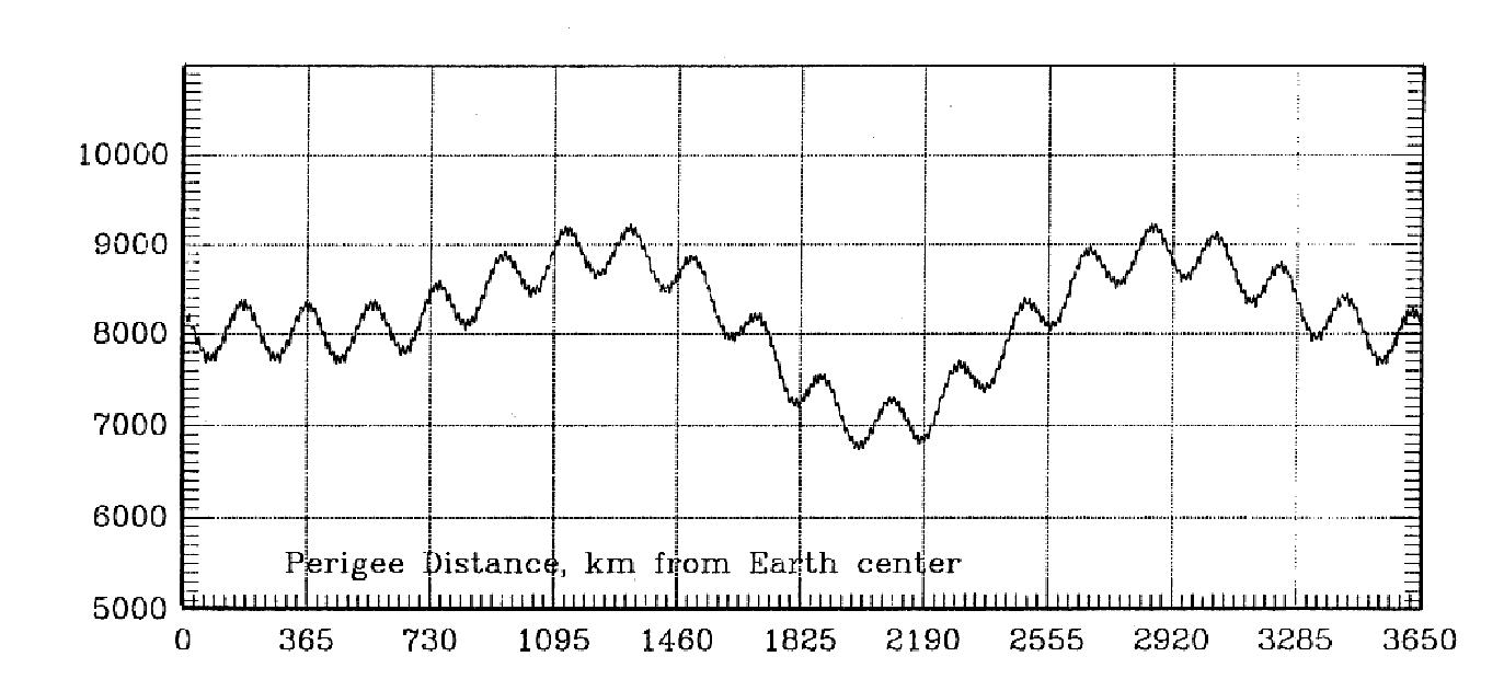
    As with magnetospheric region coverage, 12 satellites were tracked over a 2-body elliptical orbit for a 52-week year, but now their positions were checked every 10 minutes. For a 47±1 (67±1) hour orbit, satellites were placed in a downloading queue once 40 (60) hours had elapsed from their last downloading. Satellites were then handled in the order in which they entered the queue, and data acquired 56 (76) hours since the previous downloading were assumed to be lost. To be trackable by a station a satellite had to be 15° or more above its horizon and not be eclipsed.

    At the beginning of each 10-minute interval, R of each satellite being tracked was calculated. Depending on whether the 1-RE interval including R had lower limits (0, 1, 2, 3, 4) RE, it was assumed that a fraction (1, 0.625, 0.33, 0.2, 0.13) of its data accumulation was downloaded in the interval. After any downloading ended--or was interrupted by the satellite moving out of range or into an eclipse--10 minutes were allowed for switching over, after which the queue was checked and downloading was started from the satellite having the highest priority among those trackable.

    The simulations revealed that a single station would miss most of the data. For larger numbers of stations, the precentage of retrieved data is given in Table 2. The 4 locations chosen were New Mexico, Dakar, Oman and Brisbane, Australia.
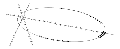
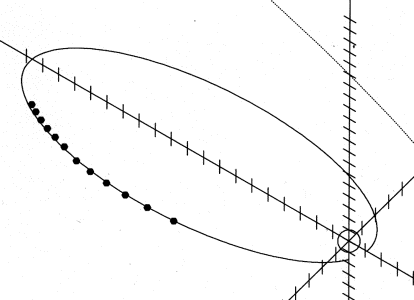

Table 2
Number   (1)   (2)   (3)
of stations . . .
2   61.3%     60.6%     50.7%  
3   79.0%     76.9%     66.8%  
4   86.5%     85.9%     75.5%  
4a   94.6%     93.4%   .

Table 2 -- The percentage of "Profile" data retrieved by 2 to 4 stations;
     4a refers to 4 stations with doubl ed sensitivity.
 Columns:
(1) For a 47±1 hr. orbit,
(2) For 67±1 hrs.,
(3) For 67±1 with 260 Mbit collected from each orbit.


It also turned out that downloading data occupied only about 7% of the stations´ time. When a group of satellites passed near Earth, the stations facing them were quite busy, but most of the time the satellites were out of range or else (30% with 4 stations, quite rare with 2 or 3) the queue was empty. This suggests that the same stations might handle more than one "constellation", or else sell surplus tracking time to other missions. Case "4a" suggests that increasing the data flow by better equipment in space or on the ground would repay handsomely

The Perturbed Orbit

Graph of perigee vs. time

An orbital code ENCKE2, based on Encke´s method [Battin, 1968; Danby, 1988] was successfully implemented, using Bulirsch-Stoer integration [Press et al.,1992, sect. 16.4]. Its output matched that of the "Swingby" commercial code and also the work by Mullins and Evans [1996] using a different Encke code GRAVE.

Orbital lifetime depends primarily on the evolution of perigee height, itself dominated by changes of the eccentricity e (perturbations leave the semi-major axis a practically constant). An initial orbit with high perigee may postpone atmospheric reentry, but it carries a heavy launch weight penalty. A better strategy is to launch into a relatively low perigee, but select an orbit whose perturbations raise it away from the atmosphere. That was the strategy of Russia´s Interball whose perigee rose from 1.2 RE to 3 RE over a single year, after it was launched at a near-critical inclination of 62.82°. Unfortunately, such high inclination would give "Profile" a rather poor plasma sheet coverage.

A typical plot of the variation of perigee height over a 10-year period is shown in Figure 4. Two main scales are evident in the 47±1 (67±1) hour orbit, a semi-annual wave of about 500 (900) km peak-to-peak and a slow long-term change. This curve, driven by variations of the eccentricity, is relatively robust, that is, raising or lowering the launch point by (say) 500 km yields a rather similar curve, but one that is displaced up or down by the appropriate amount.

That suggests a strategy for choosing the launch date: start near the time when the graph is at its lowest. Given the year of launch, that means launching at a minimum of the semi-annual wave; if a longer lead time is available, launch at a minimum when the long-term trend is also at its lowest. For a 47±1 hour "Profile" mission, a launch around the year 2007 seems optimal, with initial perigee of about 7000 km (1.1 RE).

The long-term variation of the inclination to the ecliptic was already discussed. Another question concerns the persistence of the 1-hour separation between satellites in the absence of on-board propulsion (though much of the scientific work could also adapt to shifting separations). Even a small difference in the orbital period would add up and modify this spacing, but it turns out that perturbations leave the period almost intact. Slow changes still do occur, but the simulations suggests that at least over the first 2 years, the spacing does not change greatly.

Summary

Studies of 6+6 satellites with full orbital perturbations have begun, and the design was also examined by the Integrated Mission Design Center (IMDC) at Goddard Space Flight Center. So far all plans appear feasible. The current design with mass of 17 kg seems reasonable, perhaps even conservative. The design of the mother ship is perhaps the hardest part. It requires 3-axis stabilization, rotation by 90°, extension of two arms carrying small rockets, spin-up by those rockets and accurately timed releases of pairs of satellites.

The scientific rationale and specific observation tasks for "Profile" are described in a seaparate article [Stern. 1998]. They suggest that here is a mission which could revitalize solar-terrestial research and solve or address many outstanding questions. Whether it comes to pass, and when, is up to the vision of the science community and its funding agencies.

References

  Battin, Richard H., Astronautical Guidance, xiv+400 pp, McGraw-Hill, 1964.

  Danby, John M.A., Fundamentals of Celestial Mechanics, 2nd edition, Willman-Bell, Richmond, Va., 1988.

  Mullins, Larry D. and Steven W. Evans, The Dynamics of the Proposed Orbit for the AXAF Satellite, J. Astronaut. Sci., 44, 39- 62, 1996.

  Press, William H., Saul A. Teukolsky, William T. Vetterling and Brian P. Flannery, Numerical Recipes, 2nd edition, Cambridge Univ. Press., 1992.

  Stern, D.P., The Art of Mapping the Magnetosphere, J. Geophys. Res., 99, 17,169-198, 1994.

  Stern, D.P., A Brief History of Magnetospheric Physics During the Space Age, Rev. Geophys., 34, 1-31, 1996a

  Stern, D.P., Developing a Strategy for Magnetospheric Research, Eos, 77, 165, 168, 1996b.

  Stern, D.P., Science Tasks for "Profile", 1998, this volume.


      Back to the "Profile" Index Page

Back to the "Exploration" Index Page

The author welcomes comments and suggestions, to be sent to
david("at" symbol)phy6.org.

Reformatted 10.29.99, moved to new location 1-21-2006